AI playing AirHockey
Using Model-Based Reinforcement Learning for playing AirHockey
Throughout the last years algorithms of Machine Learning have provided surprising solutions to problems in all kinds of scientific fields, from engineering to medicine and social sciences. As we in the Lab strive to make our demos even more realistic and convincing, this blog post will look at how the algorithm behind the currently used Air Hockey Demonstrator can be replaced by a truly learning AI.
Background
The problem of controlling the robotic opponent follows a game-like structure: An agent is expected to independently choose actions in order to achieve a certain goal. Therefore, we looked at this problem in the context of Reinforcement Learning, where an agent is trained to take actions in an unknown environment, guided by a reward system, which rewards or punishes the agent for taking a specific action in a certain game state.
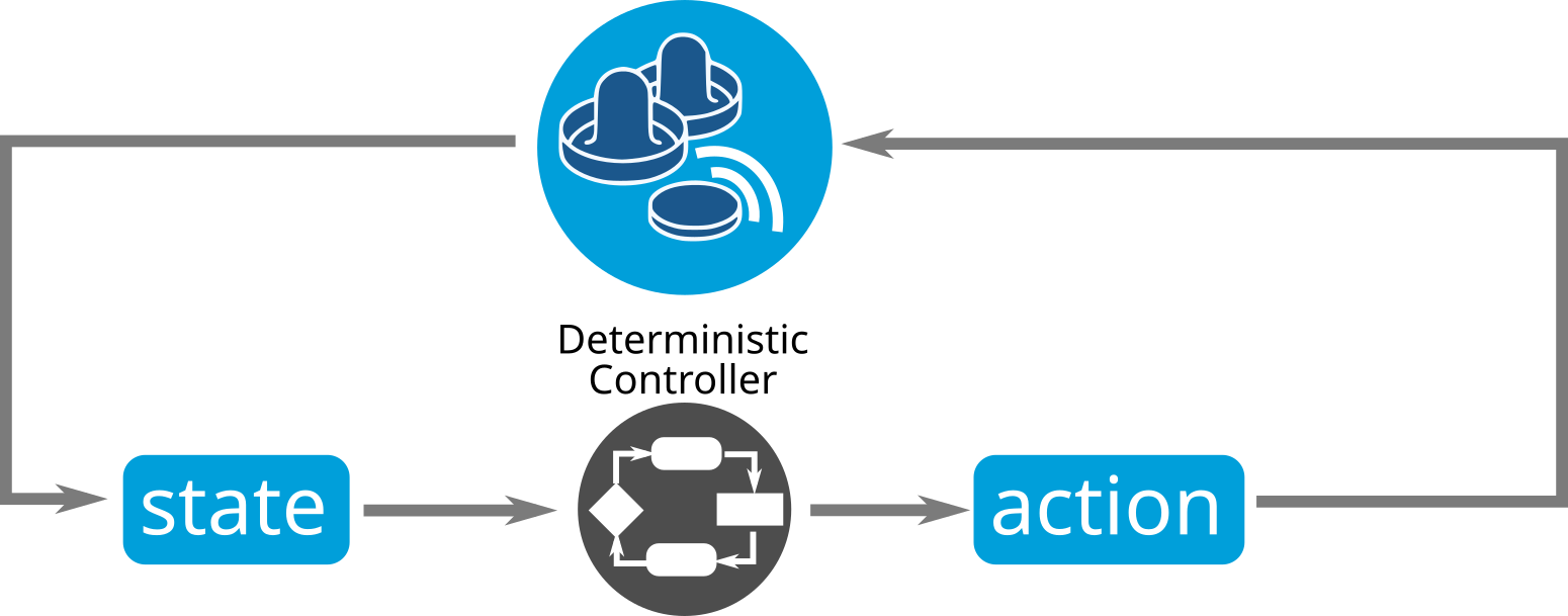 The control loop looks like this, with a deterministic hand-crafted algorithm as the controller
Classical Reinforcement Learning optimizes the trained network by trial and error, which tends to be very sample-inefficient. Due to the fact that the simulation of the Air Hockey table only runs in real-time, we chose a Model-Based Reinforcement Learning approach, namely the paper "Neural Network Dynamics for Model-Based Deep Reinforcement Learning with Model-Free Fine-Tuning" as a guideline for our implementations.
First, a so-called Dynamics Model of the environment should be learned via Supervised Learning. This network uses the current state and action applied to it to predict the following state.
Afterwards, a Model Predictive Control (MPC) controller can make use of the Dynamics Model when evaluating which action to execute. To do so, it samples a random set of possible actions and looks for the most rewarding one. Later on, this MPC can be used to initialize an action policy via Behavioral Cloning, which can be furthermore improved using classical Model-Free Reinforcement Learning algorithms.
Implementation
The Implementation was done in Python using the package pandas for evaluating the data before pre-processing,
the Keras API built on top of TensorFlow v2.0 for training and predicting with the neural network and the
package numpy throughout the project for all array-based operations.
Sample Collection
At first we need to ensure that we provide a profound data set. This data will be recorded from a game between two instances of the current deterministic robot controller which are playing against each other. With an incoming samples rate of around 200 samples/s, we record around 5 million samples per robot instance. One sample includes the state of the simulation from the perspective of one robot (position coordinates of the puck and the robot) and the action (position difference and speed) applied by the robot in this moment.
Data Pre-Processing
The data is sliced into game episodes due to the fact that the position of the puck is reset if the puck does not move for too long. In order to give the neural network a sense for time, a sliding window is used to generate the input of the network such that we will obtain a set of consecutive state-action pairs associated with an output label. Furthermore, a sliding window is applied to the differential outputs as well to be able to predict state changes for longer than just the next 5 ms.
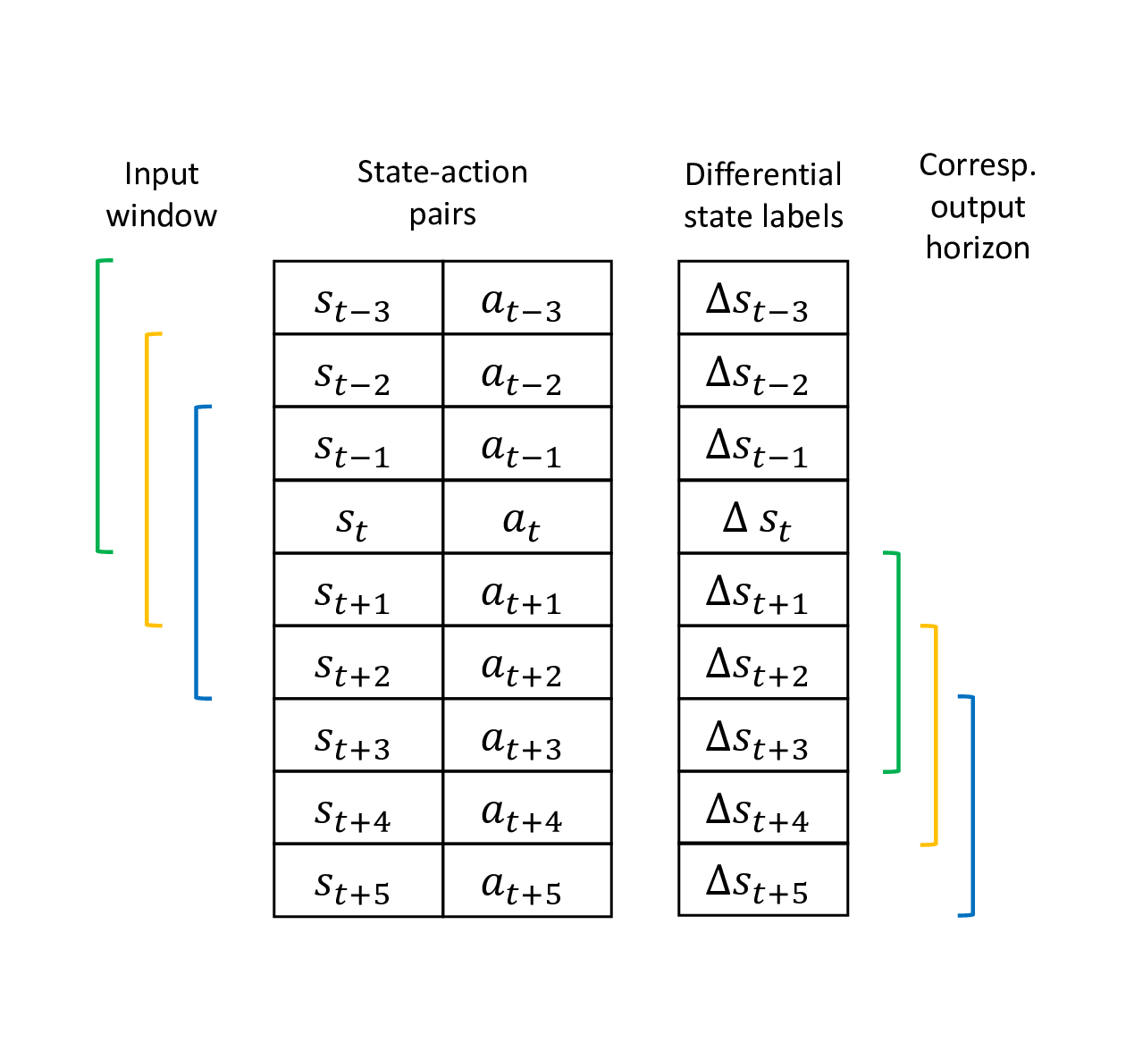
This output horizon can additionally be reduced to only obtain the differences to every n-th state into the future. Therefore, all differences along the way have to be added up as shown below.
# Reduce windowed horizon to predict only the n-th element.
# Therefore, all state differences in between these elements have to be summed up cumulatively.

curr_reduced_horizon_output = []
for i in range(len(curr_extended_horizon_output)):

    # Reshape full-horizon output window
    reshaped_horizon = np.reshape(curr_extended_horizon_output[i], (output_horizon, 4))

    reduced_horizon = []
    cumulative_diff = [0, 0, 0, 0]

    for x in range(len(reshaped_horizon)):
        # Append cumulative differences if we have reached the n-th element of the horizon vector
        if (x + 1) % reduction_factor == 0:
            reduced_horizon.append(cumulative_diff)
        # If not, keep on adding up the state differences
        else:
            cumulative_diff = [sum(i) for i in zip(cumulative_diff, reshaped_horizon[x])]

    curr_reduced_horizon_output.append(np.concatenate(reduced_horizon))
Training
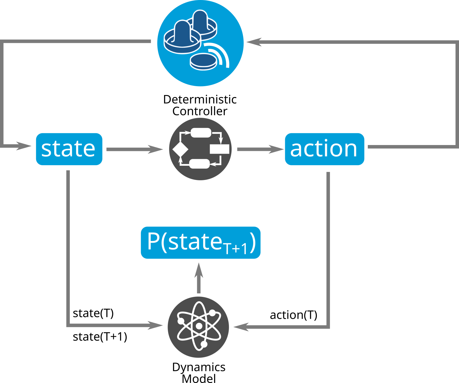 In literature the Dynamics Model is also called a Transition Model, wich determines the outcome of an action
Before the neural network is trained, the approximately 1 million samples that are left after pre-processing are split into a
- training (70%),
- validation (15%) and
- test set (15%)
A model was instantiated using the Sequential model
of the Keras API, which can be easily extended by stacking up arbitrary numbers of layers with different
configurations. In this setup we used Dense layers to build a classical fully-connected network.
# Create model
self.model = tf.keras.models.Sequential()

# Add input layer
self.model.add(tf.keras.layers.Dense(self.depth, input_dim=self.input_shape[1], activation='relu'))

# Add arbitrary number of hidden layers
for i in range(self.num_hidden - 1):
    self.model.add(tf.keras.layers.Dense(self.depth, activation='relu'))

# Add output layer
self.model.add(tf.keras.layers.Dense(self.output_shape[1]))
Further configurations of the training process are shown below:
- Input neurons: 8 x
window_size - Output neurons: 4 x
horizon_size/reduction_factor - Loss function: Mean Squared Error (MSE)
- Optimizer: Adam
- Batch size: 512
- Epochs: 30
Regarding the size of the hidden layers, the experiments first started with two layers of 500 neurons each, but we then gradually reduced the network size while maintaining a similarly good performance. Down below some examples are listed that were examined w.r.t. the network's prediction metrics and prediction latency.
| Input Window | Output Window | Reduction Factor | Hidden Layers | Total Trainable Parameters | Final Training MSE | Final Validation MSE | Test MSE | Mean Prediction Latency in ms |
|---|---|---|---|---|---|---|---|---|
| 100 | 50 | 50 | 1x 150 neurons | 120,754 | 1.4 x 1e-3 | 1.5 x 1e-3 | 1.57 x 1e-3 | 3.93 |
| 100 | 50 | 50 | 2x 50 neurons | 42,804 | 1.4 x 1e-3 | 1.5 x 1e-3 | 1.39 x 1e-3 | 3.55 |
| 100 | 50 | 10 | 1x 150 neurons | 123,170 | 0.76 x 1e-3 | 0.82 x 1e-3 | 0.77 x 1e-3 | 4.46 |
| 200 | 200 | 50 | 1x 150 neurons | 242,566 | 4 x 1e-3 | 3.8 x 1e-3 | 4.1 x 1e-3 | 7.49 |
| 200 | 200 | 50 | 2x 100 neurons | 171,816 | 3.7 x 1e-3 | 3.4 x 1e-3 | 3,54 x 1e-3 | 6.35 |
It can clearly be seen that a network with multiple smaller-sized layers is as accurate as one with only a single layer, which holds more neurons. In addition, the smaller network predicts faster due to the reduced amount of trainable parameters. As the prediction latency is a crucial constraint of our implementation, it is recommended to use this multi-layer approach.
Visualization
In order to make the prediction procedure and the network's error metrics more intuitive, an additional interface visualizes how the network is working while simultaneously displaying live state observations and the error metrics over the currently observed plotting window.
The following video shows a network with two hidden layers of 50 neurons each, using an input window of 100, an output horizon of 50 and an reduction factor of 50. Therefore, it uses around 500 ms of input samples to predict one single future state in approximately 250 ms.
A multi-horizon prediction is visualized in the following video. The only difference to the previous example is that with a reduction factor of 25, we will predict every 25th sample of the 50-sample horizon. This results in two state predictions, one at 125 ms, another at around 250 ms.
MPC
The MPC controller will now use the learned Dynamics Model to choose the most rewarding action from a set of possible actions.
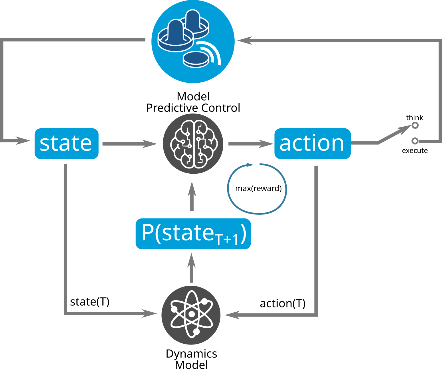 The MPC uses the Dynamics Model much like we humans simulate actions and their outcome in our brain before executing it. We tried different strategy generation and exploration methods.
Therefore, the reward system has to be defined at first. In the table below the rewards that were used for the following investigations are displayed.
| Case | Received Reward | Further Description | Possible Drawbacks |
|---|---|---|---|
| AI scores a goal | + 1.0 | Puck position in certain range close to opponent‘s goal | - |
| Opponent scores a goal | - 1.0 | Puck position in certain range close to AI‘s goal | - |
| When puck in AI's half court, decrease distance to puck | + 0.05 x (1 - distance) | - | AI might get stuck with the puck at one border |
| Puck is behind the AI | - 0.1 | puck_x > robot_x | AI could just move back to be on the same level as the puck to avoid negative reward |
| Detect a collision between robot and puck | + 0.1 | - | AI might approach the puck slowly and stop before actually hitting it, harvesting all the reward. |
| Discourage approaching the puck slowly | - 0.1 x (v_max - v) | This reward will only be evaluated if a collision was detected. If the AI stands still while colliding with the puck, it will cancel out the collision reward. | - |
| Punish puck standing still | - 0.025 | - | - |
As previously mentioned, the final implementation has certain latency constraints. Thus, a crucial factor of the MPC is how the range of possible actions will be determined because we only have a limited amount of time in which the controller is able to calculate a decision. In the following two approaches for action sampling will be described: random sampling from a discretized uniform distribution and deterministic sampling.
Random Sampling
For the random approach we first have to specify the possible range of action values that can be extracted from the implementation of the robot controller:
speed_x: 0 to 1437 mm/sspeed_y: 0 to 1475 mm/sposDiff_x: - 311 to 311 mmposDiff_x: - 295 to 295 mm
The MPC controller will randomly select actions from these discrete sets of values and choose the most rewarding one.
In the video below this random sampling approach can be seen for an amount of 20 actions evaluated per iteration. From time to time the robot seem to approach the puck on purpose, but in most cases it moves around aimlessly. This is due to the fact that the amount of evaluated, randomly chosen actions is still too small to find a rewarding strategy.
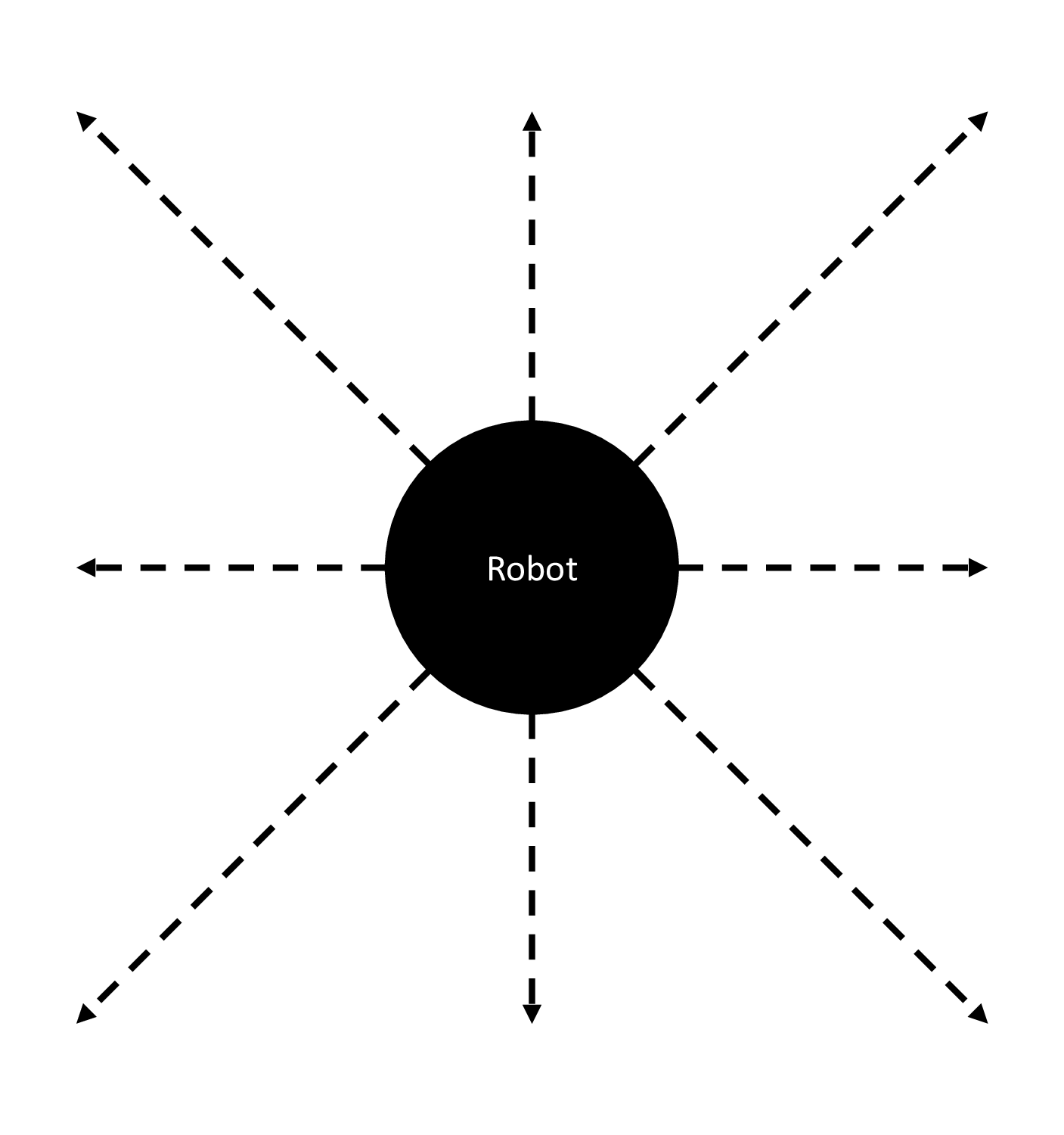
Deterministic Sampling
Another approach is to make use of our knowledge about the game's environment and its constraints in terms of possible velocities and achievable changes in position in order to limit the amount of possible actions to be checked by the MPC and therefore improve its performance. This deterministic approach assumes that we only have 8 directions (each separated by 45°) in which the robot may be able to move. The actions corresponding to these directions have to be chosen carefully in order to let the robot move there on time. Therefore, the maximum achievable puck and robot speed values have to be evaluated based on the recorded data set. It was found that the puck's maximum speed ranges around 10 m/s, letting it move across the table (1 m x 0.5 m) in around 100 ms. The robot moves at a maximum speed of 2.5 m/s in y direction, it needs to move approximately 10 to 15 cm to block the puck effectively.
Thus, the possible action values were assigned as shown below.
speed_x: 1437 mm/sspeed_y: 1475 mm/sposDiff_x: +- 100 mmposDiff_x: +- 100 mm
This approach also does not achieve the desired performance. Also, the robot sometimes seems to be stuck at the border of the area where it is allowed to move (311 x 295 mm).
Alternative: Behavioral Cloning
The implementation of the MPC did not yet achieve promising results due to the sparse amount of actions that can be evaluated because of the game's real-time constraints. But what if we could directly train a network to imitate the recorded game of both FSM-based AIs playing against each other?
As a proof of concept, this was done by first adjusting the data pre-processing such that we now use a window of
consecutive states as input (instead of state-action pairs) and the chosen actions as labels. A fully-connected network
of two hidden layers of 100 neurons each was trained for 50 epochs using a batch size of 512. The training error only
yields a final test MSE of 1.667 x 10^2, but when letting the network take control of one robot, the results look more
promising than those of the previous MPC-based implementations.
In the video it can be seen that the robot does not seem to make any attempt for an attack, but it successfully defends the goal against its opponent. This learned policy is not sufficient enough yet, but could be a promising initialization for a Model-Free Reinforcement Learning algorithm based on Policy Gradient optimization such as TRPO or PPO.
Conclusion
Our goal was to improve the performance of the robot controller, make it more resilient with better strategies.
As it turned out, having the MPC and a neural network (dynamics model) in the control loop is not fast enough under our latency constraints.
In the end, the straight forward and integrated behavioral cloning method indicated a possible way out.
Interestingly, when we tested this, using an LSTM network didn't show a better performance in dealing with time than the simple Feed Forward network.
Next Steps
From here, it would be interesting to investigate if the behavioral cloning approach could be elevated to reinforced learning by playing against each other.